# Import required libraries, grouped by functionality
# --- System and utility packages ---
from datetime import timedelta
import dotenv
import os
import requests
from zipfile import ZipFile
# --- Data handling and scientific computing ---
import math
import numpy as np
import pandas as pd
# --- Geospatial and multi-dimensional raster data ---
import geopandas as gpd
import h5py
import rasterio as rio # work with geospatial raster data
import rioxarray as rxr # work with raster arrays
from shapely import geometry
from shapely.geometry.polygon import orient
from osgeo import gdal # work with raster and vector geospatial data
import xarray as xr
# --- Plotting and visualization ---
import holoviews as hv
import hvplot.xarray # plot multi-dimensional arrays
import seaborn as sns
from matplotlib import pyplot as plt
import folium
# --- neonutilities ---
import neonutilities as nuTree Classification with NEON Airborne Imaging Spectrometer Data using Python xarray
Download, explore, interactively visualize, and perform a supervised classification using NEON AOP bidirectional reflectance data and TOS vegetation structure data.
Summary
The National Ecological Observatory Network (NEON) Airborne Observation Platform (AOP) collects airborne remote sensing data, including hyperspectral reflectance data, over 81 sites across the United States and Puerto Rico. In this notebook we will show how to download and visualize reflectance data from NEON’s Smithsonian Environmental Research Center site (SERC) in Maryland. We will then demonstrate how to run a supervised classification using the NEON Observational System (OS) Vegetation Structure data as training data, and evaluate the model results.
Background
The NEON Imaging Spectrometer (NIS) is an airborne imaging spectrometer built by JPL (AVIRIS-NG) and operated by the National Ecological Observatory Network’s (NEON) Airborne Observation Platform (AOP). NEON’s hyperspectral sensors collect measurements of sunlight reflected from the Earth’s surface in 426 narrow (~5 nm) spectral channels spanning wavelengths between ~ 380 - 2500 nm. NEON’s remote sensing data is intended to map and answer questions about a landscape, with ecological applications including identifying and classifying plant species and communities, mapping vegetation health, detecting disease or invasive species, and mapping droughts, wildfires, or other natural disturbances and their impacts.
In 2024, NEON started producing bidirectional reflectance data products (including BRDF and topographic corrections). These are currently available for AOP data collected between 2022-2025. For more details on this newly revised data product, please refer to the tutorial: Introduction to Bidirectional Hyperspectral Reflectance Data in Python.
NEON surveys sites spanning the continental US, during peak phenological greenness, capturing each site 3 out of every 5 years, for most terrestrial sites. AOP’s Flight Schedules and Coverage provide’s more information about the current and past schedules.
More detailed information about NEON’s airborne sampling design can be found in the paper: Spanning scales: The airborne spatial and temporal sampling design of the National Ecological Observatory Network.
Set Up Python Environment
No Python setup requirements if connected to the workshop Openscapes cloud instance!
Local Only
Using your preferred command line interface (command prompt, terminal, etc.) navigate to your local copy of the repository, then type the following to create a compatible Python environment.
For Windows:

```cmd
conda create -n neon_aop -c conda-forge --yes python=3.10 fiona=1.8.22 gdal hvplot geoviews rioxarray rasterio geopandas jupyter jupyter_bokeh jupyterlab h5py spectral scikit-image scikit-learn seaborn neonutilities
```

For MacOSX:

```cmd
conda create -n neon_aop -c conda-forge --yes python=3.10 gdal=3.7.2 hvplot geoviews rioxarray rasterio geopandas fiona=1.9.4 jupyter jupyter_bokeh jupyterlab h5py spectral scikit-image scikit-learn seaborn neonutilities
```
Create a NEON AOP Token
- NEON API Token (optional, but strongly recommended), see NEON API Tokens Tutorial for more details on how to create and set up your token in Python (and R). Once you create your token (on the NEON User Accounts) page, this notebook will show you how to set it as an environment variable and use it for downloading AOP data.
Optional: Download NEON Shapefiles
The lesson shows how to programmatically download the NEON shapefiles, but you can also download them by clicking on the following links:
- AOP Flight Box Boundaries: AOP_FlightBoxes.zip
- TOS Sampling Boundaries: TOS_SamplingBoundaries.zip
Learning Objectives
- Explore NEON airborne and field (instrumented, observational) shapefiles to understand what colloated data are available
- Use the neonutilities package to determine available reflectance data and download
- Use a custom function to convert reflectance data into an xarray dataset
- Create some interactive visualizations of reflectance data
- Run a random forest model to classify trees using reflectance data and data generated from vegetation structure (as the training data set)
- Evaluate classification model results
- Understand data QA considerations and potential steps to improve classification results
Tutorial Outline
- Setup
- Visualize NEON AOP, OS, and IS shapefiles at SERC
- Find available NEON reflectance data at SERC and download
- Read in and visualize reflectance data interactively
- Create a random forest model to predict the tree families from the reflectance spectra
1. Setup
1.1 Import Python Packages
If not already installed, install the neonutilities and python-dotenv packages using pip as follows: - !pip install neonutilities - !pip install python-dotenv
1.2 Set your NEON Token
Define your token. You can set this up on your NEON user account page, https://data.neonscience.org/myaccount. Please refer to the NEON API Tokens Tutorial for more details on how to create and set up your token in Python (and R).
# method 1: set the NEON_TOKEN directly in your code
NEON_TOKEN='YOUR_TOKEN_HERE'
# method 2: set the token as an environment variable using the dotenv package
dotenv.set_key(dotenv_path=".env",
key_to_set="NEON_TOKEN",#
value_to_set="YOUR_TOKEN_HERE")
# to retrieve the token that you set as an environment variable, use:
NEON_TOKEN=os.environ.get("NEON_TOKEN")2. Visualize NEON AOP, OS, and IS shapefiles at SERC
In this next section, we will look at some of the NEON spatial data, honing in on our site of interest (SERC). We will look at the AOP flight box (the area over which the NEON AOP platform flies, including multiple priority boxes), the IS tower airshed, and the OS terrestrial sampling boundaries. This will provide an overview of how the NEON sites are set up, and the spatial overlap between the field and airborne data.
First, let’s define a function that will download data from a url. We will use this to download shapefile boundares of the NEON AOP flight boxes, as well as the IS and OS shapefiles in order to see the spatial extent of the various data samples that NEON collects.
# function to download data stored on the internet in a public url to a local file
def download_url(url,download_dir):
    if not os.path.isdir(download_dir):
        os.makedirs(download_dir)
    filename = url.split('/')[-1]
    r = requests.get(url, allow_redirects=True)
    file_object = open(os.path.join(download_dir,filename),'wb')
    file_object.write(r.content)
2.1 NEON AOP flight box boundary
Download, Unzip, and Open the shapefile (.shp) containing the AOP flight box boundaries, which can also be downloaded from NEON Spatial Data and Maps. Read this shapefile into a geodataframe, explore the contents, and check the coordinate reference system (CRS) of the data.
# Download and Unzip the NEON Flight Boundary Shapefile
aop_flight_boundary_url = "https://www.neonscience.org/sites/default/files/AOP_flightBoxes_0.zip"
# Use download_url function to save the file to a directory
os.makedirs('./data/shapefiles', exist_ok=True)
download_url(aop_flight_boundary_url,'./data/shapefiles')
# Unzip the file
with ZipFile(f"./data/shapefiles/{aop_flight_boundary_url.split('/')[-1]}", 'r') as zip_ref:
    zip_ref.extractall('./data/shapefiles')
aop_flightboxes = gpd.read_file("./data/shapefiles/AOP_flightBoxes/AOP_flightboxesAllSites.shp")
aop_flightboxes.head()Next, let’s examine the AOP flightboxes polygons at the SERC site.
site_id = 'SERC'
aop_flightboxes[aop_flightboxes.siteID == site_id]
We can see the site geodataframe consists of a single polygon, that we want to include in our study site (sometimes NEON sites may have more than one polygon, as there are sometimes multiple areas, with different priorities for collection).
# write this to a new variable called "site_polygon"
site_aop_polygon = aop_flightboxes[aop_flightboxes.siteID == site_id]
# subset to only include columns of interest
site_aop_polygon = site_aop_polygon[['domain','siteName','siteID','sampleType','flightbxID','priority','geometry']]
# rename the flightbxID column to flightboxID for clarity
site_aop_polygon = site_aop_polygon.rename(columns={'flightbxID':'flightboxID'})
site_aop_polygon # display site polygon
Next we can visualize our region of interest (ROI) and the exterior boundary polygon containing ROIs.
Now let’s define a function that uses folium to display the bounding box polygon on a map. We will first use this function to visualize the AOP flight box polygon, and then we will use it to visualize the IS and OS polygons as well.
def plot_folium_shapes(
    shapefiles,      # list of file paths or GeoDataFrames
    styles=None,     # list of style dicts for each shapefile
    names=None,      # list of names for each shapefile
    map_center=None, # [lat, lon]
    zoom_start=12
):
    import pyproj
    # If no center is provided, use the centroid of the first shapefile (projected)
    if map_center is None:
        if isinstance(shapefiles[0], str):
            gdf = gpd.read_file(shapefiles[0])
        else:
            gdf = shapefiles[0]
        # Project to Web Mercator (EPSG:3857) for centroid calculation
        gdf_proj = gdf.to_crs(epsg=3857)
        centroid = gdf_proj.geometry.centroid.iloc[0]
        # Convert centroid back to lat/lon
        lon, lat = gpd.GeoSeries([centroid], crs="EPSG:3857").to_crs(epsg=4326).geometry.iloc[0].coords[0]
        map_center = [lat, lon]

    m = folium.Map(
        location=map_center,
        zoom_start=zoom_start,
        tiles=None
    )
    folium.TileLayer(
        tiles='https://mt1.google.com/vt/lyrs=y&x={x}&y={y}&z={z}',
        attr='Google',
        name='Google Satellite'
    ).add_to(m)

    for i, shp in enumerate(shapefiles):
        if isinstance(shp, str):
            gdf = gpd.read_file(shp)
        else:
            gdf = shp
        style = styles[i] if styles and i < len(styles) else {}
        layer_name = names[i] if names and i < len(names) else f"Shape {i+1}"
        folium.GeoJson(
            gdf,
            name=layer_name,
            style_function=lambda x, style=style: style,
            tooltip=layer_name
        ).add_to(m)

    folium.LayerControl().add_to(m)
    return m
map1 = plot_folium_shapes(
shapefiles=[site_aop_polygon],
names=['NEON AOP Flight Bounding Box']
)
map1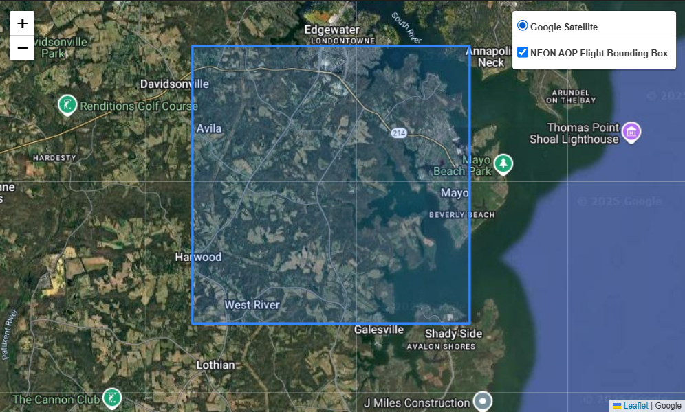
2.2 NEON OS terrestrial sampling boundaries
We will follow a similar process to download and visualize the NEON OS terrestrial sampling boundaries. The OS terrestrial sampling boundaries are also available as a shapefile, which can be downloaded from NEON Spatial Data and Maps page.
# Download and Unzip the NEON Terrestrial Field Sampling Boundaries Shapefile
neon_field_boundary_file = "https://www.neonscience.org/sites/default/files/Field_Sampling_Boundaries_202503.zip"
# Use download_url function to save the file to the data directory
download_url(neon_field_boundary_file,'./data/shapefiles')
# Unzip the file
with ZipFile(f"./data/shapefiles/Field_Sampling_Boundaries_202503.zip", 'r') as zip_ref:
zip_ref.extractall('./data/shapefiles')neon_terr_bounds = gpd.read_file("./data/shapefiles/Field_Sampling_Boundaries/terrestrialSamplingBoundaries.shp")
neon_terr_bounds.head()# save the boundaries for the site to a new variable called "site_terr_bounds"
site_terr_bounds = neon_terr_bounds[neon_terr_bounds.siteID == site_id]
site_terr_bounds.head()2.3 NEON IS tower footprint boundaries
Lastly, we’ll download and read in the IS tower footprint shapefile, which represents the area of the airshed over which the IS tower collects data. This shapefile is available from the NEON Spatial Data and Maps page, but is pre-downloaded for convenience.
# unzip the 90 percent footprint tower airshed file
with ZipFile(f"./data/90percentfootprint.zip", 'r') as zip_ref:
    zip_ref.extractall('./data/shapefiles')
# read in the neon tower airshed polygon shapefile and display
neon_tower_airshed = gpd.read_file("./data/shapefiles/90percentfootprint/90percent_footprint.shp")
neon_tower_airshed.head()# save the boundaries for the site to a new variable called "site_terr_bounds"
site_tower_bounds = neon_tower_airshed[neon_tower_airshed.SiteID == site_id]
site_tower_bounds.head()2.4 Visualize AOP, OS, and IS boundaries together
Now that we’ve read in all the shapefiles into geodataframes, we can visualize them all together as follows. We will use the plot_folium_shapes function defined above, and define a styles list of dictionaries specifying the color, so that we can display each polygon with a different color.
neon_shapefiles = [site_aop_polygon, site_terr_bounds, site_tower_bounds]

# define a list of styles for the polygons
# each style is a dictionary with 'fillColor' and 'color' keys
styles = [
    {'fillColor': '#228B22', 'color': '#228B22'}, # green
    {'fillColor': '#00FFFFFF', 'color': '#00FFFFFF'}, # blue
    {'fillColor': '#FF0000', 'color': '#FF0000'}, # red
    {'fillColor': '#FFFF00', 'color': '#FFFF00'}, # yellow
]

map2 = plot_folium_shapes(
    shapefiles=neon_shapefiles,
    names=['NEON AOP Flight Bounding Box', 'NEON Terrestrial Sampling Boundaries', 'NEON Tower Airshed'],
    styles=styles
)

map2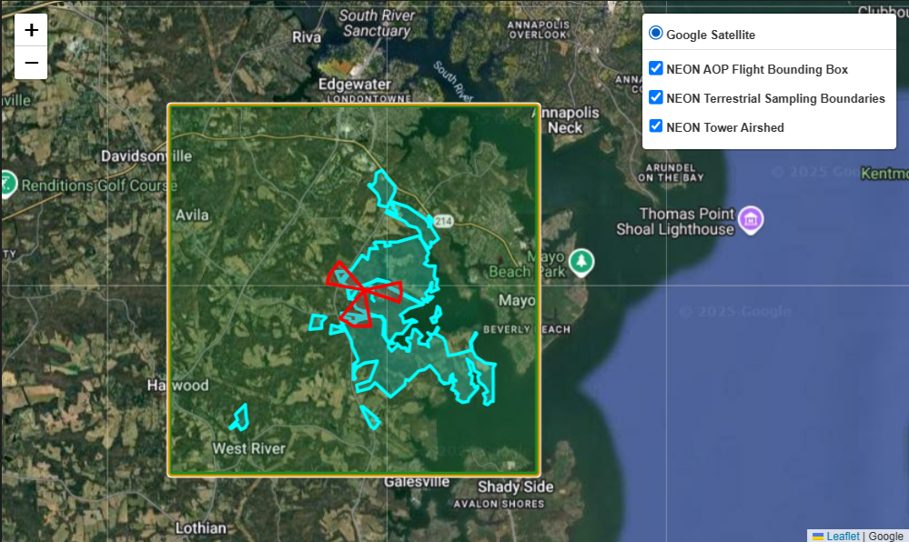
Above we can see the SOAP flightbox, and the exterior TOS boundary polygon which shows the extent of the area where observational data are collected.
3. Find available NEON reflectance data and download
Finally we can look at the available NEON hyperspectral reflectance data, which are delivered as 1 km by 1 km hdf5 files (also called tiles) over the site. The next figure we make will make it clear why the files are called tiles. First, we will determine the available reflectance data, and then pull in some metadata shapefiles from another L3 AOP data product, derived from the lidar data.
NEON hyperspectral reflectance data are currently available under two different revisions, as AOP is in the process of implementing a BRDF (Bidirectional Reflectance Distribution Function), but this has not been applied to the full archive of data yet. These data product IDs are DP3.30006.001 (directional surface reflectance), and DP3.30006.002 (bidirectional surface reflectance). The bidirectional surface reflectance data include BRDF and topographic corrections, which helps correct for differences in illumination throughout the flight.
3.1 Find available data
Let’s see what data are available at the SERC site for each of these data products using the neonutilities list_available_dates function as follows:
# define the data product IDs for the reflectance data
refl_rev1_dpid = 'DP3.30006.001'
refl_rev2_dpid = 'DP3.30006.002'print(f'Directional Reflectance Data Available at NEON Site {site_id}:')
nu.list_available_dates(refl_rev1_dpid,site_id)print(f'Bidirectional Reflectance Data Available at NEON Site {site_id}:')
nu.list_available_dates(refl_rev2_dpid,site_id)The dates provided are the year and month that the data were published (YYYY-MM). A single site may be collected over more than one month, so this publish date typically represents the month where the majority of the flight lines were collected. There are released directional reflectance data available from 2016 to 2021, and provisional bidirectional reflectance data available in 2022 and 2025. As of 2025, bidirectional data are only available provisionally because they were processed in 2024 (there is a year lag-time before data is released to allow for time to review for data quality issues).
For this exercise, we’ll look at the most recent data, from 2025. You may wish to consider other factors, for example if you collected field data in a certain year, you are looking at a year when there was a recent disturbance, or if you want to find the clearest weather data (data are not always collected in optimal sky conditions). For SERC, the most recent clear (<10% cloud cover) weather collection to date was in 2017, so this directional reflectance data may be another good option to consider for your analysis.
For this lesson, we will use the 2025 bidirectional reflectance data, which is provisional.
year = '2025'3.2 Download NEON Lidar data using neonutilities by_file_aop
We can download the reflectance data either using the neonutilities function nu.by_file_aop, which downloads all tiles for the entire site for a given year, or nu.by_tile_aop. To figure out the inputs of these functions, you can type nu.by_tile_aop?, for example.
AOP data are projected into a WGS84 coordinate system, with coordinates in UTM x, y. When using nu.by_tile_aop you need to specify the UTM easting and northing values for the tiles you want to download. If you’re not sure the extent of the site, you can use the function nu.get_aop_tile_extents. Let’s do that here, for the SOAP site collected in 2024.You will use the same token you defined at the beginning of the tutorial
serc2025_utm_extents = nu.get_aop_tile_extents(refl_rev2_dpid,
                                               site_id,
                                               year,
                                               token=NEON_TOKEN)
The AOP collection over SERC in 2025 extends from UTM 358000 - 370000 m (Easting) and 4298000 - 4312000 m (Northing). To display a list of the extents of every tile, you can print serc2025_utm_extents. This is sometimes useful when trying to determine the extents of irregularly shaped sites.
We can also look at the full extents by downloading one of the smaller lidar raster data products to start. The L3 lidar data products include metadata shapefiles that can be useful for understanding the spatial extents of the individual files that comprise the data product. To show how to look at these shapefiles, we can download the Canopy Height Model data (DP3.30015.001). The next cell shows how to do this:
# download all CHM tiles (https://data.neonscience.org/data-products/DP3.30015.001)
nu.by_file_aop(dpid='DP3.30015.001', # Ecosystem Structure / CHM
               site=site_id,
               year=year,
               include_provisional=True,
               token=NEON_TOKEN,
               savepath='./data')
The function below displays all of the folders that we’ve downloaded. You can also use your File Explorer to look at the contents of what you have downloaded.
def find_data_subfolders(root_dir):
    """
    Recursively finds subfolders within a directory that contain data (files)
    and excludes subfolders that only contain other subfolders.

    Args:
        root_dir: The path to the root directory to search.

    Returns:
        A list of paths to the subfolders containing data.
    """
    data_subfolders = []
    for root, dirs, files in os.walk(root_dir):
        # Check if the current directory has both subdirectories and files
        if dirs and files:
            # Iterate through subdirectories to find those that contain files
            for dir_name in dirs:
                dir_path = os.path.join(root, dir_name)
                if any(os.path.isfile(os.path.join(dir_path, f)) for f in os.listdir(dir_path)):
                    data_subfolders.append(dir_path)
        # If the current directory has no subdirectories, but has files, we still want to keep the directory.
        elif files:
            if root != root_dir:  # Avoid adding the root directory itself if it has files
                data_subfolders.append(root)

    return data_subfolders
# use the find_data_subfolders function to see what has been downloaded
chm_subfolders = find_data_subfolders(r'./data/DP3.30015.001')
chm_subfolders # display the subfolders# see the path of the zip file that was downloaded (ends in .zip):
for root, dirs, files in os.walk(r'./data/DP3.30015.001'):
for name in files:
if name.endswith('.zip'):
print(os.path.join(root, name)) # print file name# unzip the lidar tile boundary file
# uncomment if you skipped the download section, and comment the next line (starting with "with ZipFile")
# with ZipFile(f"./data/shapefiles/2025_SERC_7_TileBoundary.zip", 'r') as zip_ref:
with ZipFile(f"./data/DP3.30015.001/neon-aop-provisional-products/2025/FullSite/D02/2025_SERC_7/Metadata/DiscreteLidar/TileBoundary/2025_SERC_7_TileBoundary.zip",'r') as zip_ref:
zip_ref.extractall('./data/shapefiles/2025_SERC_7_TileBoundary')# read in the tile bounadry shapefile
aop_tile_boundaries = gpd.read_file("./data/shapefiles/2025_SERC_7_TileBoundary/shps/NEON_D02_SERC_DPQA_2025_merged_tiles_boundary.shp")# append this last boundary file to the existing neon_shapefiles list
neon_shapefiles.append(aop_tile_boundaries)
# plot all NEON SERC shapefiles together
map3 = plot_folium_shapes(
shapefiles=neon_shapefiles,
names=['NEON AOP Flight Bounding Box', 'NEON Terrestrial Sampling Boundaries', 'NEON Tower Airshed', 'AOP Tile Boundaries'],
styles=styles,
zoom_start=12
)
map3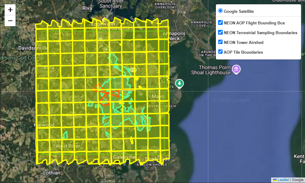
From the image above, you can see why the data are called “tiles”! The individual tiles make up a grid comprising the full site. These smaller areas make it easier to process the large data, and allow for batch processing instead of running an operation on a huge file, which might cause memory errors.
3.3 Download NEON Reflectance Data using neonutilities by_tile_aop
Now that we’ve explored the spatial extent of the NEON airborne data, as well as the OS terrestrial sampling plots and the IS tower airshed, we can start playing with the data! First, let’s download a single tile to start. For this exercise we’ll download the tile that encompasses the NEON tower, since there is typically more OS sampling in the NEON tower plots. The tile of interest for us is 365000_4305000 (note that AOP tiles are named by the SW or lower-left coordinate of the tile).
You can specify the download path using the savepath variable. Let’s set it to a data directory in line with the root directory where we’re working, in this case we’ll set it to ./data/NEON/refl.
The reflectance data are large in size (especially for an entire site’s worth of data), so by default the download functions will display the expected download size and ask if you want to proceed with the download (y/n). The reflectance tile downloaded below is ~ 660 MB in size, so make sure you have enough space on your local disk (or cloud platform) before downloading. If you want to download without being prompted to continue, you can set the input variable check_size=False.
By default the files will be downloaded following the same structure that they are stored in on Google Cloud Storage, so the actual data files are nested in sub-folders. We encourage you to navigate through the data/DP3.30006.002 folder, and explore the additional metadata (such as QA reports) that are downloaded along with the data.
# download the tile that encompasses the NEON tower
nu.by_tile_aop(dpid='DP3.30006.002',
               site=site_id,
               year=2025,
               easting=364005,
               northing=4305005,
               include_provisional=True,
               token=NEON_TOKEN,
               savepath='./data')
You can either navigate to the download folder in File Explorer, or to programmatically see what files were downloaded, you can display the files as follows:
# see all files that were downloaded (including data, metadata, and READMEs):
for root, dirs, files in os.walk(r'./data/DP3.30006.002'):
    for name in files:
        print(os.path.join(root, name))  # print file name
You can see there are several .txt and .csv files in addition to the .h5 data file (NEON_D02_SERC_DP3_364000_4305000_bidirectional_reflectance.h5). These include citation information: citation_DP3.30006.002_PROVISIONAL.txt, an issue log: issueLog_DP3.30006.002.csv, and a README: NEON.D02.SERC.DP3.30006.002.readme.20250719T050120Z.txt. We encourage you to look through these files, particularly the issue log, which conveys information about issues and the resolution for the data product in question. Make sure there is not a known issue with the data you downloaded, especially since it is provisional.
If you only want to see the names of the .h5 reflectance data you downloaded, you can modify the code as follows:
# see only the .h5 files that were downloaded
for root, dirs, files in os.walk(r'./data/DP3.30006.002'):
    for name in files:
        if name.endswith('.h5'):
            print(os.path.join(root, name))  # print file name
Success! We’ve now downloaded a NEON bidirectional surface reflectance tile into our data directory.
4. Read in and visualize reflectance data interactively
4.1 Convert Reflectance Data to an xarray Dataset
The function below will read in a NEON reflectance hdf5 dataset and export an xarray dataset. According to the xarray documentation, “xarray makes working with labelled multi-dimensional arrays in Python simple, efficient, and fun!” rioxarray is simply the rasterio xarray extension, so you can work with xarray for geospatial data.
def aop_h5refl2xarray(h5_filename):
    """
    Reads a NEON AOP reflectance HDF5 file and returns an xarray.Dataset with reflectance and weather quality indicator data.

    Parameters
    ----------
    h5_filename : str
        Path to the NEON AOP reflectance HDF5 file.

    Returns
    -------
    dsT : xarray.Dataset
        An xarray Dataset containing:
            - 'reflectance': DataArray of reflectance values (y, x, wavelengths)
            - 'weather_quality_indicator': DataArray of weather quality indicator (y, x)
            - Coordinates: y (UTM northing), x (UTM easting), wavelengths, fwhm, good_wavelengths
            - Metadata attributes: projection, spatial_ref, EPSG, no_data_value, scale_factor, bad_band_window1, bad_band_window2, etc.
    """
    import h5py
    import numpy as np
    import xarray as xr

    with h5py.File(h5_filename) as hdf5_file:
        print('Reading in ', h5_filename)
        sitename = list(hdf5_file.keys())[0]
        h5_refl_group = hdf5_file[sitename]['Reflectance']
        refl_dataset = h5_refl_group['Reflectance_Data']
        refl_array = refl_dataset[()].astype('float32')

        # Transpose and flip reflectance data
        refl_arrayT = np.transpose(refl_array, (1, 0, 2))
        refl_arrayT = refl_array[::-1, :, :]

        refl_shape = refl_arrayT.shape
        wavelengths = h5_refl_group['Metadata']['Spectral_Data']['Wavelength'][:]
        fwhm = h5_refl_group['Metadata']['Spectral_Data']['FWHM'][:]

        # Weather Quality Indicator: transpose and flip to match reflectance
        wqi_array = h5_refl_group['Metadata']['Ancillary_Imagery']['Weather_Quality_Indicator'][()]
        wqi_arrayT = np.transpose(wqi_array, (1, 0))
        wqi_arrayT = wqi_array[::-1, :]

        # Collect metadata
        metadata = {}
        metadata['shape'] = refl_shape
        metadata['no_data_value'] = float(refl_dataset.attrs['Data_Ignore_Value'])
        metadata['scale_factor'] = float(refl_dataset.attrs['Scale_Factor'])
        metadata['bad_band_window1'] = h5_refl_group.attrs['Band_Window_1_Nanometers']
        metadata['bad_band_window2'] = h5_refl_group.attrs['Band_Window_2_Nanometers']
        metadata['projection'] = h5_refl_group['Metadata']['Coordinate_System']['Proj4'][()].decode('utf-8')
        metadata['spatial_ref'] = h5_refl_group['Metadata']['Coordinate_System']['Coordinate_System_String'][()].decode('utf-8')
        metadata['EPSG'] = int(h5_refl_group['Metadata']['Coordinate_System']['EPSG Code'][()])

        # Parse map info for georeferencing
        map_info = str(h5_refl_group['Metadata']['Coordinate_System']['Map_Info'][()]).split(",")
        pixel_width = float(map_info[5])
        pixel_height = float(map_info[6])
        x_min = float(map_info[3]); x_min = int(x_min)
        y_max = float(map_info[4]); y_max = int(y_max)
        x_max = x_min + (refl_shape[1]*pixel_width); x_max = int(x_max)
        y_min = y_max - (refl_shape[0]*pixel_height); y_min = int(y_min)

        # Calculate UTM coordinates for x and y axes
        x_coords = np.linspace(x_min, x_max, num=refl_shape[1]).astype(float)
        y_coordsT = np.linspace(y_min, y_max, num=refl_shape[0]).astype(float)

        # Flag good/bad wavelengths (1=good, 0=bad)
        good_wavelengths = np.ones_like(wavelengths)
        for bad_window in [metadata['bad_band_window1'], metadata['bad_band_window2']]:
            bad_indices = np.where((wavelengths >= bad_window[0]) & (wavelengths <= bad_window[1]))[0]
            good_wavelengths[bad_indices] = 0
        good_wavelengths[-10:] = 0

        # Create xarray DataArray for reflectance
        refl_xrT = xr.DataArray(
            refl_arrayT,
            dims=["y", "x", "wavelengths"],
            name="reflectance",
            coords={
                "y": ("y", y_coordsT),
                "x": ("x", x_coords),
                "wavelengths": ("wavelengths", wavelengths),
                "fwhm": ("wavelengths", fwhm),
                "good_wavelengths": ("wavelengths", good_wavelengths)
            }
        )

        # Create xarray DataArray for Weather Quality Indicator
        wqi_xrT = xr.DataArray(
            wqi_arrayT,
            dims=["y", "x"],
            name="weather_quality_indicator",
            coords={
                "y": ("y", y_coordsT),
                "x": ("x", x_coords)
            }
        )

        # Create xarray Dataset and add metadata as attributes
        dsT = xr.Dataset({
            "reflectance": refl_xrT,
            "weather_quality_indicator": wqi_xrT
        })
        for key, value in metadata.items():
            if key not in ['shape', 'extent', 'ext_dict']:
                dsT.attrs[key] = value

        return dsT
Now that we’ve defined a function that reads in the reflectance hdf5 data and exports an xarray dataset, we can apply this function to our downloaded reflectance data. This should take around 15 seconds or so to run.
%%time
# uncomment the line below and comment the following one if running from the Openscapes platform and you skipped the download step
# serc_refl_h5 = serc_refl_h5 = r'../../shared-public/data/neon/NEON_D02_SERC_DP3_364000_4305000_bidirectional_reflectance.h5'
serc_refl_h5 = r'./data/DP3.30006.002/neon-aop-provisional-products/2025/FullSite/D02/2025_SERC_7/L3/Spectrometer/Reflectance/NEON_D02_SERC_DP3_364000_4305000_bidirectional_reflectance.h5'
serc_refl_xr = aop_h5refl2xarray(serc_refl_h5)
Next let’s define a function that updates the neon reflectance xarray dataset to apply the no data value (-9999), set the bad bands to NaN, and applies the CRS to make the xarray objet an rioxarray object. These could also be incorporated into the function above, but you may wish to work with unscaled reflectance data, for example, so we will keep these functions separate for now.
def update_neon_xr(neon_refl_ds):

    # Set no data values (-9999) equal to np.nan
    neon_refl_ds.reflectance.data[neon_refl_ds.reflectance.data == -9999] = np.nan

    # Scale by the reflectance scale factor
    neon_refl_ds['reflectance'].data = ((neon_refl_ds['reflectance'].data) /
                                        (neon_refl_ds.attrs['scale_factor']))

    # Set "bad bands" (water vapor absorption bands and noisy bands) to NaN
    neon_refl_ds['reflectance'].data[:,:,neon_refl_ds['good_wavelengths'].data==0.0] = np.nan

    neon_refl_ds.rio.write_crs(f"epsg:{neon_refl_ds.attrs['EPSG']}", inplace=True)

    return neon_refl_ds
Apply this function on our xarray dataset.
serc_refl_xr = update_neon_xr(serc_refl_xr)4.2 Visualize the reflectance dataset
Display the dataset. You can use the up and down arrows to the left of the table (e.g. to the left of Dimensions, Coordinates, Data variables, etc.) to explore each part of the dataset in more detail. You can also click on the icons to the right to see more details.
serc_refl_xr# function to auto-scale to make RGB images more realistic
def gamma_adjust(rgb_ds, bright=0.2, white_background=False):
array = rgb_ds.reflectance.data
gamma = math.log(bright)/math.log(np.nanmean(array)) # Create exponent for gamma scaling - can be adjusted by changing 0.2
scaled = np.power(np.nan_to_num(array,nan=1),np.nan_to_num(gamma,nan=1)).clip(0,1) # Apply scaling and clip to 0-1 range
if white_background == True:
scaled = np.nan_to_num(scaled, nan = 1) # Set NANs to 1 so they appear white in plots
rgb_ds.reflectance.data = scaled
return rgb_ds4.3 Plot the reflectance dataset
Now let’s plot a true color (or RGB) image of the reflectance data as shown in the cell below.
# Plot the RGB image of the SERC tower tile
serc_refl_rgb = serc_refl_xr.sel(wavelengths=[650, 560, 470], method='nearest')
serc_refl_rgb = gamma_adjust(serc_refl_rgb,bright=0.3,white_background=True)

serc_rgb_plot = serc_refl_rgb.hvplot.rgb(y='y',x='x',bands='wavelengths',
                         xlabel='UTM x',ylabel='UTM y',
                         title='NEON AOP Reflectance RGB - SERC Tower Tile',
                         frame_width=480, frame_height=480)

# Set axis format to integer (no scientific notation)
serc_rgb_plot = serc_rgb_plot.opts(
    xformatter='%.0f',
    yformatter='%.0f'
)

serc_rgb_plot
4.4 Plot the weather quality indicator data
We can look at the weather conditions during the flight by displaying the weather_quality_indicator data array. This is a 2D array with values ranging from 1 to 3, where: 1 = <10% cloud cover, 2 = 10-50% cloud cover, 3 = >50% cloud cover. NEON uses a stop-light convention to indicate the weather and cloud conditions, where green (1) is good, yellow (2) is moderate, and red (3) is poor. The figure below shows some examples of these three conditions as captured by the flight operators during science flights.
Let’s visualize this weather quality indicator data for this SERC tile using a transparent color on top of our RGB reflectance plot, following the same stop-light convention.
# Prepare the WQI mask
wqi = serc_refl_xr.weather_quality_indicator

# Map WQI values to colors: 1=green, 2=yellow, 3=red, 0/other=transparent
wqi_colors = ['#228B22', '#FFFF00', '#FF0000']
# wqi_mask = wqi[wqi > 0]  # mask out zeros or nodata

# Use hvplot with categorical colormap and alpha (50% transparency)
wqi_overlay = wqi.hvplot.image(
    x='x', y='y', cmap=wqi_colors,
    clim=(1, 3), colorbar=False, alpha=0.5,
    xlabel='UTM x', ylabel='UTM y',
    title='NEON AOP Reflectance Weather Quality - SERC Tower Tile',
    frame_width=480, frame_height=480)

# Overlay the RGB and WQI
(serc_rgb_plot * wqi_overlay).opts(title="RGB + Weather Quality Indicator").opts(xformatter='%.0f',
                                                                                 yformatter='%.0f')
The cloud conditions for this tile are yellow, which indicates somewhere between 10-50% cloud cover, which is moderate. This is not ideal for reflectance data, but it is still usable. As we will use this data for classification, you would want to consider how the cloud cover may impact your results. You may wish to find a clear-weather (<10% cloud cover) tile to run classification, or at a minimum compare results between the two to better understand how cloud cover impacts the model.
4.5 Plot a false color image
Let’s continue visualizing the data, next by making a False-Color image, which is a 3-band combination that shows you more than what you would see with the naked eye. For example, you can pull in SWIR or NIR bands to create an image that shows more information about vegetation health Here we will use a SWIR band (2000 nm), a NIR band (850 nm), and blue band (450 nm). Try some different band combinations on your own, remembering not to use bands that are flagged as bad (e.g. the last 10 bands, or those in the bad band windows between 1340-1445 nm and between 1790-1955 nm).
# Plot a False-Color image of the SERC tower tile
serc_refl_false_color = serc_refl_xr.sel(wavelengths=[2000, 850, 450], method='nearest')
serc_refl_false_color = gamma_adjust(serc_refl_false_color,bright=0.3,white_background=True)
serc_refl_false_color.hvplot.rgb(y='y',x='x',bands='wavelengths',
                         xlabel='UTM x',ylabel='UTM y',
                         title='NEON AOP Reflectance False Color Image - SERC Tower Tile',
                         frame_width=480, frame_height=480).opts(xformatter='%.0f', yformatter='%.0f')
4.6 Make an interactive spectral signature plot
We can also make an interactive plot that displays the spectral signature of the reflectance data for any pixel you click on. This is useful for exploring the spectral signature of different land cover types, and can help you identify which bands may be most useful for classification.
# Interactive Points Plotting
# Modified from https://github.com/auspatious/hyperspectral-notebooks/blob/main/03_EMIT_Interactive_Points.ipynb
POINT_LIMIT = 10
color_cycle = hv.Cycle('Category20')

# Create RGB Map
map = serc_refl_rgb.hvplot.rgb(x='x', y='y',
                               bands='wavelengths',
                               fontscale=1.5,
                               xlabel='UTM x', ylabel='UTM y',
                               frame_width=480, frame_height=480).opts(xformatter='%.0f', yformatter='%.0f')

# Set up a holoviews points array to enable plotting of the clicked points
xmid = serc_refl_rgb.x.values[int(len(serc_refl_rgb.x) / 2)]
ymid = serc_refl_rgb.y.values[int(len(serc_refl_rgb.y) / 2)]

x0 = serc_refl_rgb.x.values[0]
y0 = serc_refl_rgb.y.values[0]

# first_point = ([xmid], [ymid], [0])
first_point = ([x0], [y0], [0])
points = hv.Points(first_point, vdims='id')
points_stream = hv.streams.PointDraw(
    data=points.columns(),
    source=points,
    drag=True,
    num_objects=POINT_LIMIT,
    styles={'fill_color': color_cycle.values[1:POINT_LIMIT+1], 'line_color': 'gray'}
)

posxy = hv.streams.PointerXY(source=map, x=xmid, y=ymid)
clickxy = hv.streams.Tap(source=map, x=xmid, y=ymid)

# Function to build spectral plot of clicked location to show on hover stream plot
def click_spectra(data):
    coordinates = []
    if data is None or not any(len(d) for d in data.values()):
        coordinates.append(clicked_points[0][0], clicked_points[1][0])
    else:
        coordinates = [c for c in zip(data['x'], data['y'])]

    plots = []
    for i, coords in enumerate(coordinates):
        x, y = coords
        data = serc_refl_xr.sel(x=x, y=y, method="nearest")
        plots.append(
            data.hvplot.line(
                y="reflectance",
                x="wavelengths",
                color=color_cycle,
                label=f"{i}"
            )
        )
        points_stream.data["id"][i] = i
    return hv.Overlay(plots)

def hover_spectra(x,y):
    return serc_refl_xr.sel(x=x,y=y,method='nearest').hvplot.line(y='reflectance',x='wavelengths', color='black', frame_width=400)
    # return emit_ds.sel(longitude=x,latitude=y,method='nearest').hvplot.line(y='reflectance',x='wavelengths',
    #                                                                         color='black', frame_width=400)
# Define the Dynamic Maps
click_dmap = hv.DynamicMap(click_spectra, streams=[points_stream])
hover_dmap = hv.DynamicMap(hover_spectra, streams=[posxy])
# Plot the Map and Dynamic Map side by side
hv.Layout(hover_dmap*click_dmap + map * points).cols(2).opts(
    hv.opts.Points(active_tools=['point_draw'], size=10, tools=['hover'], color='white', line_color='gray'),
    hv.opts.Overlay(show_legend=False, show_title=False, fontscale=1.5, frame_height=480)
)
5. Supervised Classification Using TOS Vegetation Structure Data
In the last part of this lesson, we’ll go over an example of how to run a supervised classification using the reflectance data along with observational “vegetation structure” data. We will create a random forest model to classify the families of trees represented in this SERC tile, using species determined from the vegetation structure data product DP1.10098.001. See the notebook Make Training Data for Species Modeling from NEON TOS Vegetation Structure Dat to learn how the vegetation structure data were pre-processed to generate the training data file. In this notebook, we will just read in this file as a starting point.
Note that this is a quick-and-dirty example, and there are many ways you could improve the classification results, such as using more training data (this uses only data within this AOP tile), filtering out sub-optimal data (e.g. data collected in > 10 % cloud cover conditions, removing outliers (e.g. due to geospatial mis-match, shadowing, or other issues), tuning the model parameters, or using a different classification algorithm.
Let’s get started, first by exploring the training data.
5.1 Read in the training data
First, read in the training data csv file (called serc_2025_training_data.csv) that was generated in the previous lesson. This file contains the training data for the random forest model, including the taxonId, family, and geographic coordinates (UTM easting and northing) of the training points. Note that there was not a lot of extensive pre-processing when creating this training data, so you may want to consider ways to assess and improve the training data quality before running the model.
woody_veg_data = pd.read_csv(r"./data/serc_training_data.csv")
woody_veg_data.head()
We can use the xarray sel method to select the reflectance data corresponding to the training points. This will return an xarray dataset with the reflectance values for each band at the training point locations. As a test, let’s plot the reflectance values for the first training point, which corresponds to an American Beech tree (Fagaceae family).
# Define the coordinates of the first training data pixel
easting = woody_veg_data.iloc[0]['adjEasting']
northing = woody_veg_data.iloc[0]['adjNorthing']

# Extract the reflectance data from serc_refl_xr for the specified coordinates
pixel_value = serc_refl_xr.sel(x=easting, y=northing, method='nearest')
pixel_value.reflectance

# Plot the reflectance values for the pixel
plt.plot(pixel_value['wavelengths'].values.flatten(), pixel_value['reflectance'].values.flatten(), 'o');
As another test, we can plot the refletance value for one of the water bodies that shows up in the reflectance data. In the interactive plot, hover your mouse over one of the water bodies to see the UTM x, y coordinates, and then set those as the easting and northing, as shown below.
# Define the coordinates of the pixel over the pool in the NW corner of the site
easting = 364750
northing = 4305180

# Extract and plot the reflectance data from serc_refl_xr specified coordinates
pixel_value = serc_refl_xr.sel(x=easting, y=northing, method='nearest')
plt.plot(pixel_value['wavelengths'].values.flatten(), pixel_value['reflectance'].values.flatten(), 'o');
You can see that the spectral signature of water is quite different from that of vegetation.
Now that we’ve extracted the pixel value for a single pixel, we can extract the reflectance values for all of the training data points. We will loop through the rows of the training dataframe and use the xarray.Dataset.sel method to select the reflectance values of the pixels corresponding to the same geographic location as the training data points, and then we will convert this into a pandas DataFrame for use in the random forest model.
5.2 Inspect the training data
It is good practice to visually inspect the spectral signatures of the training data, for example, as shown above, to make sure you are executing the code correctly, and that there aren’t any major outliers (e.g. you might catch instances of geographic mismatch between the terrestrial location and the airborne data, or if there was a shadowing effect that caused the reflectance values to be very low).
# Get the wavelengths as column names for reflectance
wavelengths = serc_refl_xr.wavelengths.values
wavelength_cols = [f'refl_{int(wl)}' for wl in wavelengths]

records = []

for idx, row in woody_veg_data.iterrows():
    # Find nearest pixel in xarray
    y_val = serc_refl_xr.y.sel(y=row['adjNorthing'], method='nearest').item()
    x_val = serc_refl_xr.x.sel(x=row['adjEasting'], method='nearest').item()
    # Extract reflectance spectrum
    refl = serc_refl_xr.reflectance.sel(y=y_val, x=x_val).values
    # Build record: taxonID, easting, northing, reflectance values
    record = {
        'taxonID': row['taxonID'],
        'family': row['family'],
        'adjEasting': row['adjEasting'],
        'adjNorthing': row['adjNorthing'],
    }
    # Add reflectance values with wavelength column names
    record.update({col: val for col, val in zip(wavelength_cols, refl)})
    records.append(record)
Now create a dataframe from these records, and display. You can see that the reflectance values are in columns named refl_381, refl_386, etc., and the family is in the family column.
reflectance_df = pd.DataFrame.from_records(records)
# display the updated dataframe, which now includes the reflectance values for all
reflectance_df
Display the unique taxonIDs and families represented in this training data set:
reflectance_df.taxonID.unique()reflectance_df.family.unique()Next we can manipulate the dataframe using melt to reshape the data and make it easier to display the reflectance spectra for each family. This is a helpful first step to visualizing the data and understanding what we’re working with before getting into the classification model.
After re-shaping, we can make a figure to display what the spectra look like for the different families that were recorded as part of the vegetation structure data.
# Melt (re-shape) the dataframe; wavelength columns start with 'refl_'
melted_df = reflectance_df.melt(
    id_vars=['family', 'adjEasting', 'adjNorthing'],
    value_vars=[col for col in reflectance_df.columns if col.startswith('refl_')],
    var_name='wavelength',
    value_name='reflectance'
)

# Convert 'wavelength' from 'refl_XXX' to integer
melted_df['wavelength'] = melted_df['wavelength'].str.replace('refl_', '').astype(int)

# Create a summary dataframe that aggregates statistics (mean, min, and max)
summary_df = (
    melted_df
    .groupby(['family', 'wavelength'])
    .reflectance
    .agg(['mean', 'min', 'max'])
    .reset_index()
)

plt.figure(figsize=(12, 7))

# Create a color palette
palette = sns.color_palette('hls', n_colors=summary_df['family'].nunique())

# Plot the mean reflectance spectra for each family, filling with semi-transparent color between the min and max value
for i, (family, group) in enumerate(summary_df.groupby('family')):
    # print(family)
    if family in ['Fagaceae','Magnoliaceae','Hamamelidaceae','Juglandaceae','Aceraceae']:
    # Plot mean line
        plt.plot(group['wavelength'], group['mean'], label=family, color=palette[i])
        # Plot min-max fill
        plt.fill_between(
            group['wavelength'],
            group['min'],
            group['max'],
            color=palette[i],
            alpha=0.2
        )

plt.xlabel('Wavelength')
plt.ylabel('Reflectance')
plt.title('Average Reflectance Spectra by Family \n (with Min/Max Range)')
plt.legend(title='family')
plt.tight_layout()
plt.show()
We can see that the spectral signatures for the different families have similar shapes, and there is a decent amount of spread in the reflectance values for each family. Some of this spread may be due to the cloud conditions during the time of acquisition. Reflectance values of one species may vary depending on how cloudy it was, or whether there was a cloud obscuring the sun during the collection. The random forest model may not be able to fully distinguish between the different families based on their spectral signatures, but we will see!
5.3 Set up the Random Forest Model to Classify Tree Families
We can set up our random forest model by following the steps below:
- Prepare the training data by dropping the
familycolumn and setting thefamilycolumn as the target variable. Remove the bad bands (NaN) from the reflectance predictor variables. - Split the data into training and testing sets.
- Train the random forest model on the training data.
- Evaluate the model on the testing data.
- Visualize the results.
We will need to import scikit-learn (sklearn) packages in order to run the random forest model. If you don’t have these packages installed, you can install them using !pip install scikit-learn.
from sklearn.preprocessing import LabelEncoder
from sklearn.model_selection import train_test_split
from sklearn.ensemble import RandomForestClassifier
from sklearn.metrics import classification_report, accuracy_score
5.4 Prepare and clean the training data
# 1. Prepare the Data
# Identify reflectance columns
refl_cols = [col for col in reflectance_df.columns if col.startswith('refl_')]

# Remove rows with any NaN in reflectance columns (these are the 'bad bands')
clean_df = reflectance_df.dropna(axis=1)
# re-define refl_columns after removing the ones that are all NaN
refl_cols = [col for col in clean_df.columns if col.startswith('refl_')]
# display the cleaned dataframe
clean_dfNote that we have > 360 predictor variables (reflectance values for each band), and only 100 training points, so the model may not perform very well, due to over fitting. You can try increasing the number of training points by using more of the training data, or by using a different classification algorithm. Recall that we just pulled woody vegetation data from this tile that covers the tower, and there are also data collected throughout the rest of the TOS terrestrial sampling plots, so you could pull in more training data from the other tiles as well. You would likely not need all of the reflectance bands - for example, you could take every 2nd or 3rd band, or perform a PCA to reduce the number of bands. These are all things you could test as part of your model. For this lesson, we will include all of the valid reflectance bands for the sake of simplicity.
That said, we will need to remove some of the families that are poorly represented in the training data, as they will not be able to be predicted by the model. We can do this by filtering out families that have less than 10 training points. If you leave these in, the model will not be able to predict them, and will return an error when you try to evaluate the model.
# determine the number of training data points for each family
clean_df[['taxonID','family']].groupby('family').count().sort_values('taxonID', ascending=False)
# Remove the rows where there are fewer than 10 samples
# List of families to remove
families_to_remove = ['Rosaceae', 'Pinaceae', 'Ulmaceae']
# Remove rows where family is in the families_to_remove list
clean_df = clean_df[~clean_df['family'].isin(families_to_remove)].copy()5.5 Encode the target variable
Next we need to encode the target variable (family) as integers, so that the model can work properly. Encoding is the process of converting from human-readable text (words / characters) to the byte representations used by computers. We can do this using the LabelEncoder from scikit-learn.
# Encode the Target Variable (family)
# Machine learning models require numeric targets. Use LabelEncoder:
le = LabelEncoder()
clean_df['family_encoded'] = le.fit_transform(clean_df['family'])
# Display the cleaned dataframe after encoding the target variable
clean_df[['taxonID','family','family_encoded','adjEasting','adjNorthing','refl_381','refl_2461']].head()
# Confirm that the number of unique encodings is the same as the number of unique families, as a sanity check
clean_df['family_encoded'].nunique()5.6 Split the data into training and testing sets
In this next step, we will split the data into training and testing sets. We will use 80% of the data for training and 20% for testing (this is the default split). This is a common practice in machine learning to test the performance of the model, and to ensure that the model is able to generalize to new data (e.g. you’re not over-fitting).
# Split Data into Train/Test Sets
X = clean_df[refl_cols].values
y = clean_df['family_encoded'].values

X_train, X_test, y_train, y_test = train_test_split(X, y, stratify=y, random_state=42)
5.7 Create a Random Forest Classifier Object
# Create a Random Forest Classifier object and fit it to the training data
clf = RandomForestClassifier(n_estimators=100, random_state=42)
clf.fit(X_train, y_train)
5.8 Evaluate the Model
# Determine the accuracy scores based off of the test set
y_pred = clf.predict(X_test)
print("Accuracy:", accuracy_score(y_test, y_pred))
print(classification_report(y_test, y_pred, target_names=le.classes_))
What do these accuracy metrics mean?
Precision: Of the items predicted as a given class, what fraction were actually that class?
(Precision = True Positives / (True Positives + False Positives))Recall: Of all actual items of a given class, what fraction were correctly predicted?
(Recall = True Positives / (True Positives + False Negatives))F1-score: The harmonic mean of precision and recall. It balances both metrics.
(F1 = 2 * (Precision * Recall) / (Precision + Recall))Support: The number of true instances of each class in the dataset (i.e., how many samples belong to each class).
These metrics are commonly used to evaluate classification models. Ideally we would be closer to 1 for the precision, recall, and f1-scores, which would indicate that the model is performing well. The support values indicate how many training points were used for each family, and you can see that some families have very few training points, which is likely negatively impacting the model performance.
Discussion
Great job! You now should have a fairly good grasp on working with NEON airborne and field datasets together.
What are some things you could do to improve the classification results?
Models are only as good as the underlying training data - so the better the training data (more + higher quality training data points) the better your results will be.
You could consider some of the following options:
- Increase the number of training points: Use more training data from the other plots (and use more AOP tiles). You could also collect your own additional data within the NEON site.
- Filter out sub-optimal data: Remove training points that were collected in poor weather conditions (e.g. > 10% cloud cover), or that are outliers (e.g. due to spatial mis-match, shadowing, or other issues).
- Average the reflectance values over an entire tree crown: In this example, we just pulled the reflectance values from a single pixel, but you could average the reflectance values over an entire tree crown to get a more representative value for each tree. If part of the tree is in shadow, you may want to remove that pixel from the average.
- Tune the model parameters: You can adjust the hyperparameters of the random forest model, such as the number of trees, maximum depth, and minimum samples per leaf, to improve performance.
- Use a different classification algorithm: Random forest is a good starting point, but you could also try other algorithms such as support vector machines, gradient boosting, or neural networks to see if they perform better.
Next Steps
In this example, we just scratched the surface of what you can do with NEON reflectance data. Here are some next steps you could take to further explore and analyze the data:
- Apply the model to the entire reflectance dataset: Use the trained model to predict the tree families for all pixels in the reflectance dataset, and visualize the results. You may wish to include more training data for non-tree species, since the AOP data also captures non-vegetation such as water bodies, buildings, roads, etc.
- Try out the same model on SERC AOP data that was acquired in better weather conditions: Use the reflectance data from SERC 2017, which was collected in clearer weather conditions, to see if the model performs better. Note that you may need to make some minor modifications to the
aop_h5refl2xarrayfunction to accommodate the slightly different data structure of the directional reflectance data product (2019 data is not yet available with BRDF and topographic corrections, as of August 2025). - Explore other NEON sites: Use the
neonutilitiespackage to explore reflectance data from other NEON sites, and compare the spectral signatures of different land cover types. - Add in other NEON AOP datasets: In this lesson, we only looked at the reflectance data. How might other NEON data products compliment this analysis? For example, you could look at the lidar data to get information about the structure of the vegetation, for example the Canopy Height Model (CHM) or the Digital Surface Model (DSM). You could also look at the AOP imagery data.
- Use the reflectance data for other applications: The reflectance data can be used for a variety of applications, such as mapping vegetation health, detecting disease or invasive species, and mapping droughts, wildfires, or other natural disturbances and their impacts. You could use a similar approach to explore some of these applications.
# Example Challenge Solution: Apply the model to the full AOP reflectance data tile at SERC

# 1. Prepare the data:

# Extract the reflectance array from your xarray Dataset:
refl = serc_refl_xr['reflectance'].values  # shape: (y, x, bands)
# Remove the bad bands so that we can apply the model, which only uses 363 bands
good_bands = serc_refl_xr['good_wavelengths'].values.astype(bool)
refl_good = refl[:, :, good_bands]         # shape: (y, x, n_good_bands)

# 2. Reshape for prediction:
nrows, ncols, nbands = refl_good.shape
refl_2d = refl_good.reshape(-1, nbands)

# 3. Apply the model:
# Use the trained random forest model (e.g., rf_model) to predict values for every pixel
preds = clf.predict(refl_2d)

# 4. Reshape predictions back to image (y, x):
pred_map = preds.reshape(nrows, ncols)

# 5. Create an xarray DataArray for mapping, using the coordinates from your original data:
pred_xr = xr.DataArray(
    pred_map,
    dims=('y', 'x'),
    coords={'y': serc_refl_xr['y'], 'x': serc_refl_xr['x']},
    name='classification_prediction'
)

# 6. Plot the map, using hvplot to visualize:
# pred_xr.hvplot.image(x='x', y='y', cmap='tab20', title='Random Forest Classification Map')
classes = le.classes_
print('classes:', classes)
class_labels = dict(enumerate(classes))
print('class labels:',class_labels)# Convert your prediction DataArray to a categorical type with labels:
pred_xr_labeled = pred_xr.copy()
pred_xr_labeled = pred_xr_labeled.assign_coords(
family=(('y', 'x'), np.vectorize(class_labels.get)(pred_xr.values))
)# Plot the classification map, using hvplot to visualize:
from matplotlib.colors import ListedColormap, BoundaryNorm
# Plot using hvplot with the family coordinate as the color dimension:
family_codes = np.arange(7)
family_names = classes
# Choose 7 distinct colors (can use tab10, Set1, or your own)
colors = plt.get_cmap('tab10').colors[:7] # 7 distinct colors from tab10
# Create a mapping from code to color
code_to_color = {code: colors[i] for i, code in enumerate(family_codes)}
cmap = ListedColormap([code_to_color[code] for code in family_codes])
pred_xr_labeled.hvplot.image(
x='x', y='y', groupby=[], color='family', cmap=cmap,
title='Random Forest Classification Map', frame_width=600, frame_height=600
).opts(xformatter='%.0f', yformatter='%.0f')# Optional: Create a custom colorbar for the classification map
from matplotlib.colors import ListedColormap, BoundaryNorm
fig, ax = plt.subplots(figsize=(6, 1))
fig.subplots_adjust(bottom=0.5)
# Create a colormap and norm
cmap = ListedColormap([code_to_color[code] for code in family_codes])
norm = BoundaryNorm(np.arange(-0.5, 7.5, 1), cmap.N)
# Create colorbar
cb = plt.colorbar(
plt.cm.ScalarMappable(norm=norm, cmap=cmap),
cax=ax, orientation='horizontal', ticks=family_codes
)
cb.ax.set_xticklabels(family_names,fontsize=6)
cb.set_label('Family')
plt.show()Acknowledgements
Much of this tutorial was inspired by and adapated from lessons in the NASA VITALS GitHub Repository. Thank you!